KT 에이블스쿨 7기 DX 트랙에 기자단으로 신청하기도 하였고, 복습을 통한 역량을 강화, 습득을 목적으로 작성되었음을 알려드립니다.
그럼, 복습 Let's go
레이블 인코딩(Lable encoding)
- 각 범주마다 인덱스를 붙여 수치화하는 방법
- sklearn.preprocessing 모듈을 사용한다.
- 인코딩을 할 때에는 fit-transform 메서드를 활용합니다.
items=['TV','냉장고','전자렌지','컴퓨터','선풍기','선풍기','믹서','믹서']

from sklearn.preprocessing import LabelEncoder

encoder = LabelEncoder()
encoder.fit(items) # 규칙만들기
result = encoder.transform(items)
print('result : ', result)

원-핫 인코딩(One-Hot encoding) - sklearn.preprocessing.OneHotEncoder
items=['TV','냉장고','전자렌지','컴퓨터','선풍기','선풍기','믹서','믹서']

from sklearn.preprocessing import OneHotEncoder
import numpy as np


# 먼저 숫자값으로 변환을 위해 LabelEncoder로 변환합니다.
encoder = LabelEncoder()
encoder.fit(items)
labels = encoder.transform(items)

# 2차원 데이터로 변환합니다.
labels = labels.reshape(-1,1)

# 원-핫 인코딩을 적용합니다.
oh_encoder = OneHotEncoder()
oh_encoder.fit(labels)
oh_labels = oh_encoder.transform(labels)
print('원-핫 인코딩 데이터')
print(oh_labels.toarray())
print('원-핫 인코딩 데이터 차원')
print(oh_labels.shape)
※ reshape(-1,1)이란?
: 변경된 배열의 '-1' 위치의 차원은 "원래 배열의 길이와 남은 차원으로 부터 추정"이 된다는 뜻
x = np.arange(12)
x = x.reshape(3,4)
x
>>> array([[ 0,  1,  2,  3],
       	   [ 4,  5,  6,  7],
       	   [ 8,  9, 10, 11]])


           x.reshape(-1,1)
>>> array([[ 0],
       	   [ 1],
       	   [ 2],
           [ 3],
           [ 4],
           [ 5],
           [ 6],
           [ 7],
           [ 8],
           [ 9],
           [10],
           [11]])


x.reshape(-1,2)
>>> array([[ 0,  1],
           [ 2,  3],
           [ 4,  5],
           [ 6,  7],
           [ 8,  9],
           [10, 11]])


x.reshape(-1,3)
>>> array([[ 0,  1,  2],
           [ 3,  4,  5],
           [ 6,  7,  8],
           [ 9, 10, 11]])
또 다른 방법은?
원 핫 인코딩의 pd.get_dummies() 가 있습니다.
- pd.get_dummies()를 활용하면, 데이터프레임형태의 인코딩된 결과를 얻을 수 있습니다.
import pandas as pd
import numpy as np

df = pd.DataFrame({'item':['TV','냉장고','전자렌지','컴퓨터','선풍기','선풍기','믹서','믹서'] })
피처 스케일링과 정규화
StandardScaler
- StandardScaler는 데이터의 평균을 0, 표준편차를 1로 변환하여 정규 분포 형태로 표준화합니다.
- 스케일이 다른 특성들을 동일한 기준으로 맞춰주기 위해 사용합니다.
- 학습 데이터에 fit_transform()을 적용하고, 테스트 데이터에는 transform()만 적용해야 합니다. 이렇게 해야 테스트 데이터의 정보가 학습에 반영되지 않아 데이터 누수를 방지할 수 있습니다.
from sklearn.datasets import load_iris
import pandas as pd

# 붓꽃 데이터 셋을 로딩하고 DataFrame으로 변환합니다.
iris = load_iris()
iris_data = iris.data
iris_df = pd.DataFrame(data=iris_data, columns=iris.feature_names)

print('feature 들의 평균 값')
print(iris_df.mean())
print('\nfeature 들의 분산 값')
print(iris_df.var())
from sklearn.preprocessing import StandardScaler

# StandardScaler객체 생성
scaler = StandardScaler()
# StandardScaler 로 데이터 셋 변환. fit( ) 과 transform( ) 호출.
scaler.fit(iris_df)
iris_scaled = scaler.transform(iris_df)

#transform( )시 scale 변환된 데이터 셋이 numpy ndarry로 반환되어 이를 DataFrame으로 변환
iris_df_scaled = pd.DataFrame(data=iris_scaled, columns=iris.feature_names)
print('feature 들의 평균 값')
print(iris_df_scaled.mean())
print('\nfeature 들의 분산 값')
print(iris_df_scaled.var())
MinMaxScaler
- MinMaxScaler는 데이터를 0과 1 사이의 범위로 압축하는 정규화 방식입니다.
- 특성 간의 최소값과 최대값을 기준으로 스케일을 조정하므로, 모든 특성이 동일한 범위를 가지게 된다.
- fit_transform()은 반드시 학습 데이터에만 적용하고, 테스트 데이터는 transform()만 해야 한다.
from sklearn.preprocessing import MinMaxScaler

# MinMaxScaler객체 생성
scaler = MinMaxScaler()
# MinMaxScaler 로 데이터 셋 변환. fit() 과 transform() 호출.
scaler.fit(iris_df)
iris_scaled = scaler.transform(iris_df)

# transform()시 scale 변환된 데이터 셋이 numpy ndarry로 반환되어 이를 DataFrame으로 변환
iris_df_scaled = pd.DataFrame(data=iris_scaled, columns=iris.feature_names)
print('feature들의 최소 값')
print(iris_df_scaled.min())
print('\nfeature들의 최대 값')
print(iris_df_scaled.max())
실습 프로세스
① 데이터 불러오기
② 데이터 탐색
③ 데이터 전처리
④ 학습/테스트 데이터 분리
⑤ 모델 선택 및 학습
⑥ 예측 및 평가
0. 라이브러리 불러오기
import numpy as np
import pandas as pd
import matplotlib.pyplot as plt

import warnings # 에러 안 뜨게 하는 방법!
warnings.filterwarnings(action='ignore')
1. 데이터 불러오기
- 데이터 가져와서 과정을 준비한다.
- 인코딩 방식은 'euc-kr'을 활용하세요.
- 독립 변수 데이터셋 : './data/X.csv'
- 종속 변수 데이터셋 : './data/y.csv'
x = pd.read_csv('./data/X.csv', encoding='euc-kr' )
y = pd.read_csv('./data/y.csv', encoding='euc-kr')

print(x.shape)
print(y.shape)

# (3500, 10)
# (3500, 2)
2. 데이터 탐색하기
- 데이터를 이해할 수 있도록 탐색과정을 수행해 봅시다!
먼저, 데이터의 상위 몇 개 행을 출력하여 전체 구조를 미리 확인해봅니다.
# 여기에 코드를 작성하세요

display(x.head(10))
display(y.head(10))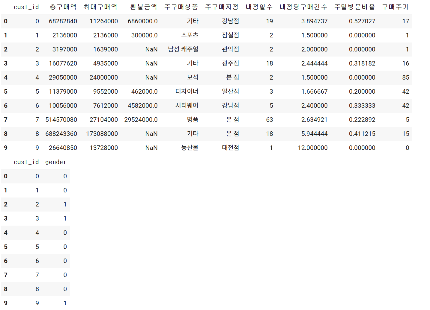
데이터의 요약 정보나 통계 정보를 출력해 변수들의 유형과 분포를 확인합니다.
※ object가 있으니깐, 인코딩해야겠다는 생각을 해야 한다.
※ 환불금액의 1205 non-null을 보고 결측치가 있다는 판단을 하고, 바로 결측치를 만들어야 한다.
※ cust_id는 인덱스랑 똑같으니 사라지게 만들어야 한다.
# 여기에 코드를 작성하세요

display(x.info())

# object 가 있으니깐 인코딩해야겠다는 생각을 해야 한다.
# 환불금액의 1205보고 결측치가 있다는 판단을 하고, 바로 결측치 처리해야 한다.
# cust_id는 인덱스랑 똑같으니 사라지게 만들어야 한다.
데이터의 요약 정보나 통계 정보를 출력해 변수들의 유형과 분포를 확인합니다.
x.describe()
데이터 전처리
- 전처리 과정을 통해서 머신러닝에 사용할 수 있는 형태의 데이터 준비
※ 인코딩, 스케일링을 수행하고, cust_id 제거, 결측치 처리
※ 결측치 처리는 0으로 대체하고, 환불금액
from sklearn.preprocessing import LabelEncoder
from sklearn.preprocessing import StandardScaler
- 단순히 1부터의 숫자를 부여한 'cust_id'를 수치형 변수로 받아드리게 된다면, 결과가 왜곡될 수 있으니깐 컬럼을 제거해봅시다.
x = x.iloc[:, 1:   ]
y = y.iloc[:, -1]

# 4장에서는 x = df_scaled[:, :-1], y = df_scaled[:, -1] 이렇게 했는데, 이건 ndarray이고
# 위 x,y는 DF 데이터 프레임이여서 df.loc, df.iloc로 불러와야 한다. (loc 문자열, iloc 숫자로 불러옴)
사라졌나 확인해 봅시다.
print(x.shape)
print(y.shape)

#(3500, 9)
#(3500,)
- 데이터에 결측치가 있는지 확인해봅시다.
x.isnull().sum()
- 환불금액에 2295개의 결측치가 있으니, 결측치에 0으로 채워 넣어서 모델 학습에 지장이 없도록 합시다!
x['환불금액'].fillna('0', inplace = True)

x.isnull().sum()
문자형 범주 데이터를 숫자로 바꾸기 위한 인토딩을 수행해 봅시다.
# x.info() 를 해서 어디에 인코더를 수행할지 한번 봐야한다. (object를 바꿔야 한다. -> 주구매상품/주구매지점 바꿈)

from sklearn.preprocessing import LabelEncoder
from sklearn.preprocessing import StandardScaler

encoder = LabelEncoder()

col_lst = ['주구매상품', '주구매지점']

for col in col_lst:
  x[col] = encoder.fit_transform(x[col])

# x['주구매상품'] = encoder.fit+transform(x['주구매상품'])
# x['주구매지점'] = encoder.fit+transform(x['주구매지점']) 과 같은 뜻이다.
학습/테스트 데이터 분리
- 데이터를 학습용과 테스트용으로 나눕니다.
from sklearn.model_selection import train_test_split

x_train, x_test, y_train, y_test = train_test_split(x, y, test_size = 0.3, random_state= 12345)

print(x_train.shape)
print(y_train.shape)
print(x_test.shape)
print(y_test.shape)'KT AIVLE > 데이터 분석, ML, DL' 카테고리의 다른 글
| [KT AIVLE DX 트랙 7기] 미니프로젝트 1차 (0) | 2025.04.20 |
|---|---|
| [KT AIVLE 스쿨 7기] 딥러닝 (0) | 2025.04.16 |
| [KT AIVLE DX 트랙 7기] 회귀학습 & 분류학습 (0) | 2025.04.13 |
| [KT AIVLE DX 트랙 7기] 인공지능과 머신러닝 (1) | 2025.04.09 |
| [KT AIVLE DX 트랙 7기] 가설검증 & 이변량 분석과 시각화 (0) | 2025.04.06 |